Review:
In previous lessons we have seen two growth models: the linear growth model and the exponential growth model.
The Linear Growth Model:
Linear growth is characterized by a fixed amount of growth between each transition.
Example. P[1] = 100, and P[n+1] = P[n] +20
Recall that the transition rule is f(x) = x + 20 because each new population level is determined by adding 20 to the previous population level. Hence P[n+1] = P[n] + 20 = f(P[n]). In general, the transition rule describing a population sequence (or any recursive sequence) is that function f(x) such that P[n+1] = f(P[n]).
|
More generally... The Linear Growth Model is any model of the form: P[n+1] = P[n] + d
|
Exponential Growth Model:
Exponential growth is characterized by a fixed percentage increase or decrease between each transition.
Example. P[1] = 100, P[n+1] = 1.2P[n]
In this example the population increases by a fixed 20 percent with each iteration. It is easy to see this when you rewrite the model into the form:
P[n+1] = 1.2P[n] = (1+0.2)P[n] = P[n] + 0.2P[n]
The population at stage n+1 is the old population, P[n], plus another 20 percent of that population, 0.2P[n].
|
More generally... The Exponential Growth Model is any model of the form: P[n+1] = r P[n] where r is some constant.
|
The Logistic Growth Model:
Exponential Growth (with r > 1) describes a situation in which there is unrestrained breeding. The population sequence grows without bound, increasing by the same percentage at each stage. Of course, this is unrealistic. Resources will eventually run out in any habitat, prohibiting such unlimited growth, so one would expect the population to eventually level off. Saying this another way, as the population increases, resources (food, space, etc) run low, and reproduction rates should decrease.
Hence, if we wish to change the exponential model P[n+1] = rP[n] to construct a more realistic model then we should change the growth factor r.
In particular, the growth factor should depend on the population level.
- When population P[n] is small, resources are plenty, and the growth factor should be large.
- When population P[n] is large, resources run low, and the growth factor should be small.
In short, the growth factor R in an improved model should be a decreasing function of P[n]. The easiest way to accomplish this is with a downsloping line:The most simple scenario... R(P[n]) is a down-sloping line:
R(P[n]) = r - mP[n], r > 0, m > 0
Example. As an example, let the growth factor R for some population model, P[n+1] = R(P[n])P[n], be described by the line: R(P[n]) = 2 - 0.2P[n], where P[n] is measured in thousands.
With this scenario the population will have a growth factor close to 2 when the population is very small (i.e., when P[n] is close to zero), because R(0) = 2 - 0.2(0) = 2. This means that, initially, the population will tend to double in size. As the population increases, however, the growth factor decreases. When P[n] is 2 (meaning 2000), the growth factor is 2 - 0.2(2) = 1.6, and the population at stage n+1 is P[n+1] = 1.6*P[n]. When P[n] is 5 the growth factor is 2 - 0.2(5) = 1, and P[n+1] = 1*P[n] = P[n]. The population remains at a level of 5 (i.e., 5000).
To examine the situation more carefully look at the table below. The table contains the population sequence described by the model P[n+1] = (2 - 0.2P[n])P[n] with initial population P[1] = .1 (in thousands).
As n increases from 1 to 10 the population approaches 5,000. Early on, the population is nearly doubling in size from one iteration to the next. As the population size approaches 5,000, however, the growth rate slows down. In fact, looking at the second column you notice that the growth factors are approaching 1 as P[n] approaches 5,000. As we saw earlier, this means that the population will start to level off, because a growth factor of 1 corresponds to a 0 increase (or decrease) in population.
n
P[n] (in thousands)
R(P[n]) = 2 - 0.2P[n]
P[n+1] = R(P[n])P[n]
1
0.1
2-0.2(0.1) = 1.9800
1.98(0.1) = 0.1980
2
0.198
2 - 0.2(0.198) = 1.9604
1.9604(0.198) = 0.3882
3
0.3882
2 - 0.2(0.3882) = 1.9224
1.9224(0.3882) = 0.7463
4
0.7463
2 - 0.2(0.7463) = 1.8507
1.8507(0.7563) = 1.3812
5
1.3812
2 - 0.2(1.3812) = 1.7238
1.7238(1.3812) = 2.3809
6
2.3809
2 - 0.2(2.3809) = 1.5238
1.5238(2.3809) = 3.6281
7
3.6281
2 - 0.2(3.6281) = 1.2744
1.2744(3.6281) = 4.6239
8
4.6239
2 - 0.2(4.6239) = 1.0753
1.0753(4.6239) = 4.9720
9
4.9720
2 - 0.2(4.9720) = 1.0056
1.0056(4.9720) = 4.9998
10
4.9998
2 - 0.2(4.9998) = 1.0000
1.0000(4.9998) = 5.0000
A graph of this population sequence might be helpful...
P[1] = 0.1, P[n+1] = (2 - 0.2P[n])P[n]
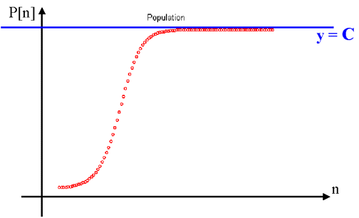
Note S-shape of the curve. The growth appears to be exponential early on, but the sequence flattens out at 5,000. Indeed, the population sequence never surpasses 5,000!
The example above illustrates a population model exhibiting logistic growth.
More generally, the Logistic Growth Model is characterized by the fact that its growth factor is described by a downsloping line, dependent on the population level. Symbolically, we say that the growth factor has the form R(P[n]) = r - mR(P[n]) where r > 0 and m > 0.
Definition.
The Logistic Growth Model is any model of the form:
P[n+1] = (r - mP[n]) P[n]
where r > 0 and m > 0.
Logistic growth is famous for its characteristic S-shape:

The value C in the graph above is known as the Carrying Capacity of the model. From a biological point of view, C represents the number of organisms that the habitat can sustain. In our earlier model, the carrying capacity was 5,000.
| Back to the Math 108 Course Schedule |
Last modified: September 22, 2007 |