Maple worksheet for implementing Euler's method 


First, call the "DEtools" and "plots" packages. 


> with(DEtools); -1; with(plots); -1


Define the differential equation that you want to study. 


> `:=`(f, proc (t, y) options operator, arrow; `+`(y, `-`(`*`(`^`(t, 2)))) end proc); 1
 

proc (t, y) options operator, arrow; `+`(y, `-`(`*`(`^`(t, 2)))) end proc (1)


Specify the initial conditions. 


> `:=`(t[0], 0); 1; `:=`(y[0], 1); 1


0
1 (2)


Specify the step size and the total number of steps that you want to take. 


> `:=`(dt, .1); 1; `:=`(N, 10); 1


.1
10 (3)


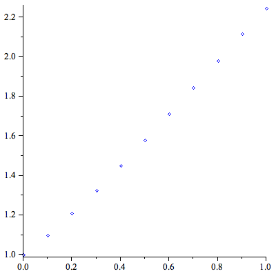
Implement the method (and create a plot of the results). 


> `:=`(euler_pts, [t[0], y[0]]); -1; for n from 0 to `+`(N, `-`(1)) do `:=`(t[`+`(n, 1)], `+`(t[n], dt)); `:=`(y[`+`(n, 1)], `+`(y[n], `*`(dt, `*`(f(t[n], y[n]))))); `:=`(new_pt, [t[`+`(n, 1)], y[`+`(n,...
`:=`(euler_pts, [t[0], y[0]]); -1; for n from 0 to `+`(N, `-`(1)) do `:=`(t[`+`(n, 1)], `+`(t[n], dt)); `:=`(y[`+`(n, 1)], `+`(y[n], `*`(dt, `*`(f(t[n], y[n]))))); `:=`(new_pt, [t[`+`(n, 1)], y[`+`(n,...


[.1, 1.1]
[.2, 1.209]
[.3, 1.3259]
[.4, 1.44949]
[.5, 1.578439]
[.6, 1.7112829]
[.7, 1.84641119]
[.8, 1.982052309]
[.9, 2.116257540]
[1.0, 2.246883294] (4)


Display the plot of the numerical results of Euler's method. 


> display(eulerPlot); 1
 

Plot_2d
 

>