Using Maple to Draw Bifurcation Diagrams
You can use Maple to help construct bifurcation diagrams. Begin by calling the "plots" package.
| > |
 |
Next, define the autonomous differential equation that you want to study.
| > |
 |
 |
(1) |
We can find the equilibrium points in Maple by solving the equation f=0 in terms of y.
| > |
 |
 |
(2) |
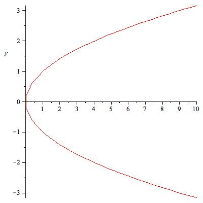
To construct the bifurcation diagram, we want to look at the values of the paramater alpha that produce equilibrium points for the differential equation. This means that we want to look at the values of alpha that make f equal to 0. The "implictplot" command generates a plot of the values of alpha and corresponding equilibrium points, as shown below.
| > |
 |
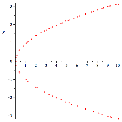
The "style=point" option generates the following type of plot:
| > |
 |
Let's look at another example. Before we begin, we should use the "restart" command in Maple.
| > |
 |
| > |
 |
 |
(3) |
| > |
 |
 |
(4) |
| > |
 |
| > |
 |
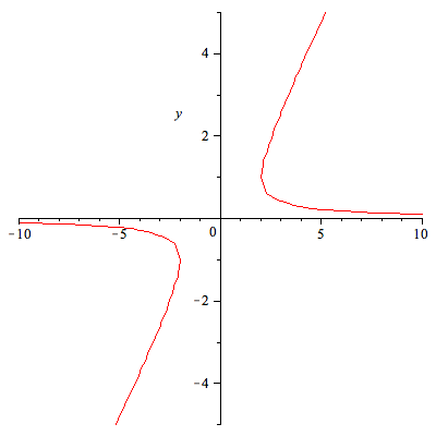
It can sometimes be useful to store the equilibrium points in Maple as expressions so that you can work with them later. For example, once you have stored the expressions for the equilibrium points (I've called them y1 and y2 below), you can use Maple to give you numerical values for the equilibrium points for different values of alpha.
| > |
 |
 |
(5) |
| > |
 |
 |
(6) |
| > |
 |
 |
(7) |
Typing "alpha:=5" and then "y1" and "y2" gives you the exact values for the equilibrium points y1 and y2 when the numerical value of alpha is 5.
| > |
 |
 |
(8) |
| > |
 |
 |
 |
(9) |
Typing "alpha:=5." (note the period after the 5) gives you numerical values for the equilibrium points y1 and y2 when the numerical value of alpha is 5. This can be helpful for sketching bifurcation diagrams.
| > |
 |
 |
(10) |
| > |
 |
 |
 |
(11) |
| > |
 |
 |
(12) |
| > |
 |
 |
 |
(13) |
| > |
 |
| > |
 |


